using Pkg
Pkg.activate("working_directory")Course
Requirements
For this course you need to have the following software installed
jupyter
a latex distribution with the following packages
- pythontex
- pgfplots
- standalone
- graphicx
- tikzscale
Data processing in julia
The basics
We’ll cover syntax and basic usage of julia by going through the intro notebooks of JuliaAcademy.
Using an environment
It is advised to use separate environments for different projects, thus we either navigate to the folder we want to work in and activate the environment with
if we want to activate the current directory we could have used ".".
If we are in a REPL we can also use pkg-mode instead:
] activate .In the following we always use the Pkg notation, but you can always also use pkg-mode instead.
When using environments provided by other people it might be neccessary to instantiate the environment which downloads all packages specified in the environment.
Pkg.instantiate()From csv data to figure
Say we got some measured data from a measuring device in csv format and lets assume the path to this file is saved in a variable called csv_path. For example if our file is in the same directory as the julia file, we can set csv_path = @__DIR__.
We can now combine the packages DataFrames.jl and CSV.jl to read the data and store it in a tabular data structure. Therefore we need to add these packages to our environment once via
Pkg.add(["DataFrames", "CSV"])We also need to take into account that the first two rows of the file are the header.
using CSV
using DataFrames

csv_path = joinpath("working_directory", "data", "scope_0.csv")
df = CSV.read(csv_path, DataFrame, header = [1,2])
2,000 rows × 2 columns
| x-axis_second | 1_Volt | |
|---|---|---|
| Float64 | Float64 | |
| 1 | -1.0e-5 | 0.0 |
| 2 | -9.99e-6 | -0.40201 |
| 3 | -9.98e-6 | 0.0 |
| 4 | -9.97e-6 | -0.40201 |
| 5 | -9.96e-6 | 0.0 |
| 6 | -9.95e-6 | 0.0 |
| 7 | -9.94e-6 | 0.40201 |
| 8 | -9.93e-6 | 0.40201 |
| 9 | -9.92e-6 | 0.0 |
| 10 | -9.91e-6 | 0.40201 |
| 11 | -9.9e-6 | 0.40201 |
| 12 | -9.89e-6 | 0.40201 |
| 13 | -9.88e-6 | 0.0 |
| 14 | -9.87e-6 | 0.40201 |
| 15 | -9.86e-6 | 0.0 |
| 16 | -9.85e-6 | 0.0 |
| 17 | -9.84e-6 | 0.0 |
| 18 | -9.83e-6 | -0.0 |
| 19 | -9.82e-6 | 0.0 |
| 20 | -9.81e-6 | -0.0 |
| 21 | -9.8e-6 | 0.0 |
| 22 | -9.79e-6 | 0.40201 |
| 23 | -9.78e-6 | 0.40201 |
| 24 | -9.77e-6 | 0.40201 |
| 25 | -9.76e-6 | 0.0 |
| 26 | -9.75e-6 | 0.0 |
| 27 | -9.74e-6 | 0.40201 |
| 28 | -9.73e-6 | 0.0 |
| 29 | -9.72e-6 | 0.0 |
| 30 | -9.71e-6 | -0.40201 |
| ⋮ | ⋮ | ⋮ |
Next, we want to create a plot from this DataFrame using Plots.jl. Thus we add Plots.jl to our environment.
Pkg.add("Plots")To plot the two columns of the data frame against each other we have to access their data. If the two columns would have been named x and y we could easily access these columns by df.x and df.y, but unfortunately they have names that are not valid identifiers in julia (the first one contains a hyphen and the second one starts with a number). Fortunately, we can get around this by using the var string macro.
using CSV
using DataFrames
using Plots

df = CSV.read(csv_path, DataFrame, header = [1,2])

plot(df.var"x-axis_second", df.var"1_Volt")
[ Info: Precompiling Plots [91a5bcdd-55d7-5caf-9e0b-520d859cae80][ Info: Precompiling GR_jll [d2c73de3-f751-5644-a686-071e5b155ba9]
Adding units
In julia it is possible to attach units to our number using Unitful.jl, additionally we can add a bit of convenience when plotting these using UnitfulRecipes.jl which defines plotting recipes for unitful quantities.
You know the game:
Pkg.add(["Unitful", "UnitfulRecipes"])
Note
As of Plots v1.35 and julia v1.9 loading UnitfulRecipes can be omitted.
using CSV
using DataFrames
using Unitful
using Plots
using UnitfulRecipes

df = CSV.read(csv_path, DataFrame, header=[1, 2])
df[!, Symbol("x-axis_second")] *= Unitful.s
df[!, Symbol("1_Volt")] *= Unitful.V

plot(df.var"x-axis_second" .|> u"μs", df.var"1_Volt")
There are some package specific notations we used:
- When indexing a
DataFramethe package distinguishes returning a copy of the data withdf[:, column]or a view withdf[!, column]. Unitful.jluses the pipe operator|>as a shortcut foruconvert, sox |> u"μs"is the same asuconvert(x, u"μs"). The dot applies this to every entry of the collection.- The plot recipes defined in
UnitfulRecipes.jlautomatically attach the units to the x- and y-axis labels.
Fine tuning plots
In this course we want to integrate our plots with a pgfplotsx-backend of Plots.jl as well as the LaTeXStrings.jl package.
Pkg.add(["PGFPlotsX", "LaTeXStrings"])Furthermore we add axis labels, change the color of the plotted line, ignore values where time is smaller than 0 and disable the legend by default. For later use in the document we save it in .tikz format in a plots folder and set tex_output_standalone to false by default.
using CSV
using DataFrames
using Unitful
using Plots
using UnitfulRecipes
pgfplotsx(legend=false, tex_output_standalone=false)

df = CSV.read(csv_path, DataFrame, header=[1, 2])
df[!, Symbol("x-axis_second")] *= Unitful.s
df[!, Symbol("1_Volt")] *= Unitful.V

plot(df.var"x-axis_second" .|> u"μs", df.var"1_Volt",
  color=colorant"#cc1188",
  xlabel=L"T",  # the L string macro creates LaTeXStrings
  ylabel=L"U",
  xlims=(0, Inf),
)
savefig(joinpath(@__DIR__, "plots", "signal.tikz")) # other locations possible
The improved plot looks like this: 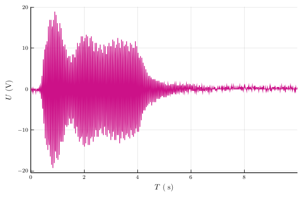
Fitting a curve
If you are noting down the values of the measurement yourself, it might be a good idea to write them down into a julia file right away.
For demonstration purposes we use a different package for a tabular data structure, namely TypedTables.jl which is a bit more minimalist than DataFrames.jl, but you could also use DataFrames.jl.
Imagine we are noting down times in ms and voltages in kV and we know that the voltage measurement has an uncertainty of 0.29 kV. We can encode this uncertainty in the number type using the package Measurements.jl.
Pkg.add(["TypedTables", "Measurements"])Let’s put the file tau-M.jl in the data folder and this is how it could look like:
using TypedTables
using Measurements

const tau_M = Table(
    var"τ[ms]" = [
        0.1 ,
        2.0 ,
        4.0 ,
        6.0 ,
        8.0 ,
        10.0,
        12.0,
        14.0,
        16.0,
        18.0,
        20.0,
        22.0,
        24.0,
        26.0,
        28.0,
        30.0,
        32.0,
        34.0,
        36.0,
        38.0,
        40.0,
        42.0,
        44.0,
        46.0,
        48.0,
        50.0,
        52.0,
        54.0,
    ],
    var"U[kV]" = [
        -8.9 ± 0.29,
        -8.1 ± 0.29,
        -7.3 ± 0.29,
        -6.5 ± 0.29,
        -5.8 ± 0.29,
        -5.1 ± 0.29,
        -4.4 ± 0.29,
        -3.8 ± 0.29,
        -3.2 ± 0.29,
        -2.5 ± 0.29,
        -1.9 ± 0.29,
        -1.35 ± 0.29,
        -0.78 ± 0.29,
        0.00 ± 0.29,
        0.54 ± 0.29,
        1.1 ± 0.29,
        1.5 ± 0.29,
        1.9 ± 0.29,
        2.3 ± 0.29,
        2.7 ± 0.29,
        3.1 ± 0.29,
        3.5 ± 0.29,
        3.8 ± 0.29,
        4.1 ± 0.29,
        4.3 ± 0.29,
        4.6 ± 0.29,
        4.8 ± 0.29,
        4.9 ± 0.29,
    ]
)
Let’s take a look at the collected data by doing a scatter plot:
using Plots
using LaTeXStrings
using Measurements
using TypedTables
pgfplotsx(legend=false, tex_output_standalone=false)

include(joinpath("working_directory", "data", "tau-M.jl"))

scatter(tau_M.var"τ[ms]", tau_M.var"U[kV]",
  markersize = 3,
  xlabel = L"\tau \textrm{[ms]}",
  ylabel = L"U \textrm{[kV]}",
  title = latexstring(raw"Messung $T_1$"),
)
Note, how the recipe defined in Measurements.jl automatically applied error-bars to our plot.
Fitting
Now lets fit this data with an exponential saturation
For this we’ll use the package LsqFit.jl and add it to our environment via
Pkg.add("LsqFit")Let’s start by writing a simple implementation of our function
expSat(x,S,b,we) = S*(1-b*exp(-x/we))Now, to make this work with LsqFit.jl we need to make sure it handles vector input and we need to be able to pass all parameters in one vector. To easily change our function to handle vector input, we can use the @. broadcast macro, which “adds a dot” to every function call afterwards (see broadcasting). For the parameters, we can add another method that unpacks the parameter vector via splatting and calls our original implementation.
expSat(x,S,b,we) = @. S*(1-b*exp(-x/we))
expSat(x, p) = expSat(x, p...)
expSat (generic function with 2 methods)Sometimes packages compose really well in julia thanks to multiple dispatch and generic algorithms. Sometimes they don’t, in our case LsqFit.jl expects only floating point values as input, so we have to extract the values of our Measurement objects. Then we can use curve_fit to do the fitting with some starting values for the parameters.
using LsqFit
fit = curve_fit(expSat, tau_M.var"τ[ms]", Measurements.value.(tau_M.var"U[kV]"), [7.0,3.0,10.0])
[ Info: Precompiling LsqFit [2fda8390-95c7-5789-9bda-21331edee243]LsqFit.LsqFitResult{Vector{Float64}, Vector{Float64}, Matrix{Float64}, Vector{Float64}}([11.519813315403889, 1.7894066440722454, 45.42829540940477], [-0.14849088381612674, -0.10598042587066203, -0.05638314137255929, -0.04337832840153233, 0.0346100644221643, 0.07909020735825134, 0.09150531321155775, 0.1732364350737945, 0.22560514356555572, 0.14987608876851555 … -0.11261159685370048, -0.11066057945833352, -0.12602174211307915, -0.1579494427742132, -0.1057301544785978, -0.0686810821351882, 0.05385116110813737, 0.06249182048839064, 0.1578392116973104, 0.3404658807469154], [-0.785472006891041 -11.494482971490584 -0.0009966567286427738; -0.7123362333535165 -11.023650664639447 -0.019116641726397317; … ; 0.43037496146950954 -3.6671229122150746 -0.16534268022209817; 0.45490892406608047 -3.5091785622918596 -0.1643067443722631], true, Float64[])We can now use the coefficients of the fit to create an anonymous function and then add an automatically sampled line to our plot by passing it to the plot! function. The bang (!) indicates that this function changes our previous plot instead of creating a new one.
plot!(x->expSat(x,coef(fit)))
Make your life easier with recipes
Plots.jl lets you define custom processing of arguments dependent on their type using so called recipes.
Let us define a recipe for Table which takes specified columns of the table and plot them against each other and also use the names of the columns as corresponding axis labels
using Plots
using TypedTables

@recipe function f(tt::Table; indices = [1,2])
  x_name, y_name = propertynames(tt)[indices]
  xlabel --> string(x_name)
  ylabel --> string(y_name)
  getproperty(tt, x_name), getproperty(tt, y_name)
end
In julia we call the definition of methods where you neither own the function nor the type type piracy. This is something you should try to avoid when possible and never put into any package. However, sometimes it comes in handy in scripts like this, where you want to extend the functionality of a package you don’t own.
After these words of warning, let’s cover the recipe syntax. This works by putting the @recipe macro in front of a function definition. The name of the function can be arbitrary. The signature then determines which type of recipe we are writing. In this case its a user recipe which is the most common type of recipe.
Inside the function you can use the two operators special operators to set plot attributes. Either a default value that will get overridden when you provide a different value in the plot call with --> or you set a value, that can’t be changed via :=. Whatever you return from the function will be used as arguments to the plot call (potentially chaining recipes).
With this we can write our second plot script as
using Plots
using LaTeXStrings
using Measurements
using TypedTables
pgfplotsx(legend=false, tex_output_standalone=false)
@recipe function f(tt::Table; indices = [1,2])
  x_name, y_name = propertynames(tt)[indices]
  xlabel --> string(x_name)
  ylabel --> string(y_name)
  getproperty(tt, x_name), getproperty(tt, y_name)
end

include(joinpath(@__DIR__, "data", "tau-M.jl"))

scatter(tau_M.var"τ[ms]", tau_M.var"U[kV]",
  markersize = 3,
  xlabel = L"\tau \textrm{[ms]}",
  ylabel = L"U \textrm{[kV]}",
  title = latexstring(raw"Messung $T_1$"),
)

fit = curve_fit(expSat, tau_M.var"τ[ms]", Measurements.value.(tau_M.var"U[kV]"), [7.0,3.0,10.0])
plot!(x->expSat(x,coef(fit)))
savefig(joinpath(@__DIR__, "plots", "t1.tikz"))
Incorporation into pythontex
Basics of pythontex
pythontex allows the execution of code blocks of several programming languages and capture the output in the created document.
In this course we are using julia and therefore we need to specify this in the package options.
\usepackage[usefamily={jl,julia,juliacon}]{pythontex}It is possible to read the documentation via texdoc pythontex.
Inline and block code execution
pythontex defines the macro \jl{} for inline evaluation of julia code and the environment jlcode for execution of blocks of julia code. The environment is used like
\begin{jlcode}
  print("Hello pythontex")
\end{jlcode}
You can have multiple sessions per document and there might be code that should be executed at the beginning of each section. For this purpose pythontex defines the pythontexcustomcode environment.
A minimal report
First steps
In the following I’ll assume the following structure of the working directory:
working_directory/
├─ data/
│  ├─ scope_0.csv
├─ plots/
│  ├─ signal.tikz
│  ├─ t1.tikz
├─ scripts/
│  ├─ signal.jl
│  ├─ t1.jl
├─ report.tex
With this in mind lets try to show one of our plots in a simple
\documentclass[a4paper]{report}

\usepackage[usefamily={jl,julia,juliacon}]{pythontex}
\usepackage{graphicx}
\usepackage{tikzscale}

%% this part of the preamble is required by the pgfplotsx backend and can be queried by calling `Plots.pgfx_preamble()` in julia
\usepackage{pgfplots}
\pgfplotsset{compat=newest}
\usepgfplotslibrary{groupplots}
\usepgfplotslibrary{polar}
\usepgfplotslibrary{smithchart}
\usepgfplotslibrary{statistics}
\usepgfplotslibrary{dateplot}
\usepgfplotslibrary{ternary}
\usetikzlibrary{arrows.meta}
\usetikzlibrary{backgrounds}
\usepgfplotslibrary{patchplots}
\usepgfplotslibrary{fillbetween}
\pgfplotsset{%
  layers/standard/.define layer set={%
    background,axis background,axis grid,axis ticks,axis lines,axis tick labels,pre main,main,axis descriptions,axis foreground
  }%
  {grid style= {/pgfplots/on layer=axis grid},%
    tick style= {/pgfplots/on layer=axis ticks},%
    axis line style= {/pgfplots/on layer=axis lines},%
    label style= {/pgfplots/on layer=axis descriptions},%
    legend style= {/pgfplots/on layer=axis descriptions},%
    title style= {/pgfplots/on layer=axis descriptions},%
    colorbar style= {/pgfplots/on layer=axis descriptions},%
    ticklabel style= {/pgfplots/on layer=axis tick labels},%
    axis background@ style={/pgfplots/on layer=axis background},%
    3d box foreground style={/pgfplots/on layer=axis foreground},%
  },
}
%%

\author{\Large{Julia Roberts} \and \Large{Julia Lang}}
\title{\Huge{$\mathtt{magnatic resonance}$}}
\date{}

\begin{document}
\maketitle

\begin{figure}
  \centering
  \includegraphics[width=\textwidth]{plots/signal.tikz}
  \caption{Signal of coil probe}
  \label{fig:signal}
\end{figure}

\end{document}
This can be compiled using lualatex report.
Computing things
In the previous example we precomputed the image and inserted it into the document. Now, we want to generate the figure while generating the document and also use the results of our fit in the text.
For this we will use a jlcode environment inside the normal figure environment like this:
\begin{figure}
  \centering
  \begin{jlcode}
    include(joinpath("..", "scripts", "t1.jl"))
    show(stdout, "application/x-tex", current())
  \end{jlcode}
  \caption{Measurement of $T_1$.}
\end{figure}
Note, that pythontex operates in its own subfolder of the current working directory, thus we have to go one level up before entering the scripts folder. Then we get the current plot with the current() function of Plots.jl and tell it to return a
Next, we want to add a sentence about the value of fit. In julia we can calculate these values via coef(fit)[3] and stderror(fit)[3], since it is the third parameter. However, if we use these values as is, we will get a lot of decimals.
coef(fit)[3], stderror(fit)[3](45.42829540940477, 2.034724167493512)Therefore, we exploit the fact, that Measurements.jl only displays the significant digits.
using Measurements
coef(fit)[3] ± stderror(fit)[3]
45.4 ± 2.0If we additionally use the latexify function of Latexify.jl we get a nice expression that we can directly use in our document:
using Measurements, Latexify
latexify(coef(fit)[3] ± stderror(fit)[3])
L"$45.4 ± 2.0$"If we put all our using statements at the beginning of our document in a pythontexcustomcode environment our document looks like this:
\documentclass[a4paper]{report}

\usepackage[usefamily={jl,julia,juliacon}]{pythontex}
\usepackage{graphicx}
\usepackage{tikzscale}

%% this part of the preamble is required by the pgfplotsx backend and can be queried by calling `Plots.pgfx_preamble()` in julia
\usepackage{pgfplots}
\pgfplotsset{compat=newest}
\usepgfplotslibrary{groupplots}
\usepgfplotslibrary{polar}
\usepgfplotslibrary{smithchart}
\usepgfplotslibrary{statistics}
\usepgfplotslibrary{dateplot}
\usepgfplotslibrary{ternary}
\usetikzlibrary{arrows.meta}
\usetikzlibrary{backgrounds}
\usepgfplotslibrary{patchplots}
\usepgfplotslibrary{fillbetween}
\pgfplotsset{%
  layers/standard/.define layer set={%
    background,axis background,axis grid,axis ticks,axis lines,axis tick labels,pre main,main,axis descriptions,axis foreground
  }%
  {grid style= {/pgfplots/on layer=axis grid},%
    tick style= {/pgfplots/on layer=axis ticks},%
    axis line style= {/pgfplots/on layer=axis lines},%
    label style= {/pgfplots/on layer=axis descriptions},%
    legend style= {/pgfplots/on layer=axis descriptions},%
    title style= {/pgfplots/on layer=axis descriptions},%
    colorbar style= {/pgfplots/on layer=axis descriptions},%
    ticklabel style= {/pgfplots/on layer=axis tick labels},%
    axis background@ style={/pgfplots/on layer=axis background},%
    3d box foreground style={/pgfplots/on layer=axis foreground},%
  },
}
%%

\author{\Large{Julia Roberts} \and \Large{Julia Lang}}
\title{\Huge{$\mathtt{magnatic resonance}$}}
\date{}

\begin{document}
  \maketitle

  \begin{pythontexcustomcode}{jl}
    using Latexify
    using Measurements
  \end{pythontexcustomcode}

\begin{figure}
  \centering
  \includegraphics[width=\textwidth]{plots/signal.tikz}
  \caption{Signal of coil probe}
  \label{fig:signal}
\end{figure}

\begin{figure}
  \centering
  \begin{jlcode}
    include(joinpath("..", "scripts", "t1.jl"))
    show(stdout, "application/x-tex", current())
  \end{jlcode}
  \caption{Measurement of $T_1$.}
  \label{fig:t1}
\end{figure}
%
From the fitting in \ref{fig:t1} results a value of $T_1 = (\jl{latexify(coef(fit)[3] ± stderror(fit)[3])}\,\mathrm{ms})$.
\end{document}
When using pythontex compilation consist of at least three steps
lualatex report
pythontex report
lualatex reportTables and statistics
Suppose we have collected additional data about frequencies data/omega_m.jl.
using DataFrames
using Unitful

omega_m_data = DataFrame(
    (ω = [
        21.3u"MHz",
        21.25u"MHz",
        21.22u"MHz",
        21.202u"MHz",
        21.192u"MHz",
    ],
    ωₘ = [
        108.3u"kHz",
        58.4u"kHz",
        28.2u"kHz",
        9.9u"kHz",
        1.5u"kHz",
    ],
    ωᵣₑₛ = [
        21.1917u"MHz",
        21.1916u"MHz",
        21.1918u"MHz",
        21.1921u"MHz",
        21.1905u"MHz",
    ])
)
We will now use PrettyTables.jl to generate a nice
Pkg.add("PrettyTables")The main interface of PrettyTables.jl is the pretty_table function and using it might look like this:
\begin{table}
  \centering
  \begin{jlcode}
    include("../data/omega_m.jl")
    pretty_table(stdout, omega_m_data, header = latexify.(propertynames(omega_m_data)), nosubheader=true, backend=Val(:latex), wrap_table=false)
  \end{jlcode}
  \caption{Measured frequencies.}
\end{table}
Using the standard library Statistics we can compute the mean and standard deviation of the resonance frequencies via
using Statistics, Measurements
include(joinpath("working_directory", "data", "omega_m.jl"))
mean(omega_m_data.ωᵣₑₛ) ± std(omega_m_data.ωᵣₑₛ)
21.19154 ± 0.00061 MHzWe add these to our report:
\documentclass[a4paper]{report}

\usepackage[usefamily={jl,julia,juliacon}]{pythontex}
\usepackage{graphicx}
\usepackage{tikzscale}

%% this part of the preamble is required by the pgfplotsx backend and can be queried by calling `Plots.pgfx_preamble()` in julia
\usepackage{pgfplots}
\pgfplotsset{compat=newest}
\usepgfplotslibrary{groupplots}
\usepgfplotslibrary{polar}
\usepgfplotslibrary{smithchart}
\usepgfplotslibrary{statistics}
\usepgfplotslibrary{dateplot}
\usepgfplotslibrary{ternary}
\usetikzlibrary{arrows.meta}
\usetikzlibrary{backgrounds}
\usepgfplotslibrary{patchplots}
\usepgfplotslibrary{fillbetween}
\pgfplotsset{%
  layers/standard/.define layer set={%
    background,axis background,axis grid,axis ticks,axis lines,axis tick labels,pre main,main,axis descriptions,axis foreground
  }%
  {grid style= {/pgfplots/on layer=axis grid},%
    tick style= {/pgfplots/on layer=axis ticks},%
    axis line style= {/pgfplots/on layer=axis lines},%
    label style= {/pgfplots/on layer=axis descriptions},%
    legend style= {/pgfplots/on layer=axis descriptions},%
    title style= {/pgfplots/on layer=axis descriptions},%
    colorbar style= {/pgfplots/on layer=axis descriptions},%
    ticklabel style= {/pgfplots/on layer=axis tick labels},%
    axis background@ style={/pgfplots/on layer=axis background},%
    3d box foreground style={/pgfplots/on layer=axis foreground},%
  },
}
%%

\author{\Large{Julia Roberts} \and \Large{Julia Lang}}
\title{\Huge{$\mathtt{magnatic resonance}$}}
\date{}

\begin{document}
  \maketitle

  \begin{pythontexcustomcode}{jl}
    using Latexify
    using Measurements
    using Statistics
    using PrettyTables
  \end{pythontexcustomcode}

\begin{figure}
  \centering
  \includegraphics[width=\textwidth]{plots/signal.tikz}
  \caption{Signal of coil probe}
  \label{fig:signal}
\end{figure}

\begin{figure}
  \centering
  \begin{jlcode}
    include(joinpath("..", "scripts", "t1.jl"))
    show(stdout, "application/x-tex", current())
  \end{jlcode}
  \caption{Measurement of $T_1$.}
  \label{fig:t1}
\end{figure}
%
From the fitting in \ref{fig:t1} results a value of $T_1 = (\jl{latexify(coef(fit)[3] ± stderror(fit)[3])}\,\mathrm{ms})$.
%
\begin{table}
  \centering
  \begin{jlcode}
    include("../data/omega_m.jl")
    pretty_table(stdout, omega_m_data, header = latexify.(propertynames(omega_m_data)), nosubheader=true, backend=Val(:latex), wrap_table=false)
  \end{jlcode}
  \caption{Measured frequencies.}
  \label{tab:omega_m}
\end{table}
%
From the measured frequency values shwon in tab.~\ref{tab:omega_m} a mean value of $\omega_{res}=\jl{latexify(mean(omega_m_data.ωᵣₑₛ) ± std(omega_m_data.ωᵣₑₛ))}$ is calculated for the resonance frequency, which is close to the guidevalue of $22.3\,\mathrm{MHz}$.
\end{document}Workflow management using make
Simple Makefile
We have accumulated quite some steps that need to be done one after the other and if we want to update our report some day in the future it is easy to forget some of it and end up with an inconsistent document.
Therefore, we will record the workflow of what needs to be done in which order to create our report in a Makefile. A Makefile has a set of rules with the following syntax
<target>: <prerequisites>
    <command>
where <target> is the file to be generated, <prerequisites> are the file(s) needed for that and the <command> is how the <target> is created. Note that <command> needs to be indented with a hard tab and not with spaces.
Our Makefile could look like this:
report.pdf: plots/signal.tikz
    lualatex report
    pythontex report
    lualatex report

plots/signal.tikz: scripts/signal.jl data/scope_0.csv
    julia scripts/signal.jl
It would then be enough to call make in the working directory to create our report. Without further arguments make will build the first rule in the file and check if any dependent files where updated to check if it needs to re-execute their rules.
Elaborate Makefile
Let’s make our Makefile a bit more useful. Imagine we were to rename the report.tex file. This would cause us to need to change the Makefile at multiple lines. Therefore, we will introduce a variable NAME:
NAME := report

$(NAME).pdf: plots/signal.tikz
    lualatex $(NAME)
    pythontex $(NAME)
    lualatex $(NAME)

plots/signal.tikz: scripts/signal.jl data/scope_0.csv
    julia $<
We also used the automatic variable $< which refers to the first prerequisite. Now we’d only need to change one line, if we changed the name of report.tex and we can also change the name on the command line with make NAME=<new name>.
Cleaning up
Since clean target to remove things when no longer needed. We don’t want to actually create a file named clean though, therefore we have to mark this target as PHONY in the Makefile.
Also we can make our lives a bit easier by using the built-in functions, which are called like this
$(<function name> <argument1>[, <optionally more arguments>])This is how our final Makefile looks like:
NAME:=report

$(NAME).pdf: plots/signal.tikz
    lualatex ${NAME} &&\
    pythontex ${NAME} &&\
    (biber ${NAME} || true) &&\
    lualatex ${NAME} &&\
    lualatex ${NAME}

plots/signal.tikz: scripts/signal.jl data/scope_0.csv
    julia --project=@. $<

.PHONY: clean
clean:
    $(foreach ending, ps log out dvi bbl blg fls fdb_latexmk pdf aux pytxcode,  rm -f ${NAME}.$(ending);)
    rm -rf pythontex-files-${NAME}
There is a lot more you can do, but this should be enough for this course.
Also checkout the make guide from The Turing Way and the documentation.
Versions
This document was generated using the following versions:
println("Julia: $VERSION")
Pkg.status()
Julia: 1.7.3 Status `/builds/comp-bio/teaching/julia-physics-report/working_directory/Project.toml` [336ed68f] CSV v0.10.4
[a93c6f00] DataFrames v1.3.4
[b964fa9f] LaTeXStrings v1.3.0
[23fbe1c1] Latexify v0.15.16
[2fda8390] LsqFit v0.12.1
[eff96d63] Measurements v2.7.2
[8314cec4] PGFPlotsX v1.5.0
[91a5bcdd] Plots v1.31.3
[08abe8d2] PrettyTables v1.3.1
[9d95f2ec] TypedTables v1.4.0
[1986cc42] Unitful v1.11.0
[42071c24] UnitfulRecipes v1.5.3Attributions
- julia icon by Stefan Karpinski under CC-BY-NC-SA 4.0